
A deep dive into the architecture, training instability, and the reality of small-scale LLMs.
You can check the source code here Med-Karim-Ben-Boubaker/gpt-2-from-scratch.
I completed my most educational project yet: building an LLM from scratch. By “from scratch,” I mean implementing the fundamental building blocks of a basic GPT‑2–style model (Radford et al., 2019) using mostly plain PyTorch. The result is an LLM that’s fluent in English, but sometimes insists that France is in Germany, or gives bizarre answers to simple geography questions like “What is the capital of Spain?”
But sometimes it surprises me with how accurate the answer is, which is not something I expected from a ~35M-parameter model:
In today’s article, I’m going to walk through the project end-to-end: the steps, the challenges, and how I did all of this on a small GPU (an RTX 3050 with only 4GB of VRAM) with ~10 hours of pre-training and ~3 hour of instruction fine-tuning.
Introduction and motivation
I’ve always admired LLM technology, and I wanted to understand its internals to better grasp its nature, so I could better understand its limitations and potential capabilities. Even after watching countless lectures and reading books, it’s important to implement the thing yourself to discover that it’s not as easy as it looks.
Most resources talk about implementation and mathematical equations, but don’t emphasize how important the data, tokenization, and training process are. Especially for a small language model, the non-architectural choices become even more important.
My first resource that helped me with the implementation of the Transformer, tokenizer, and basic training scripts was Build a Large Language Model (From Scratch) (Raschka, 2024). It also helped me understand some of the theory behind LLMs.

For more depth, especially why the Transformer exists in the first place, I highly recommend the lectures provided by CS231n: Deep Learning for Computer Vision by Stanford (focus on Lecture 8: Attention and Transformers) (Stanford CS231n, n.d.).

Let’s start by understanding the most important steps:
The processing unit of the Transformer (tokens)
Tokenization is one of the most important components in building natural language processing systems, particularly for Transformers. It represents the discretization process needed by any digital system. We can define tokenization as the transformation function that converts any continuous input (like images or human language) into discrete, independent blocks called “tokens.”
Let’s take this sentence as an example: “Many words map to one token, but some don’t: indivisible.” This represents continuous linguistic information. Humans intuitively discretize this sentence into words, resulting in a list like [Many, words, map, to, one, etc…]. We could even tokenize each word further into characters.
However, for LLMs, this basic logic is not optimized and presents several problems. We must remember that LLMs don’t necessarily see words for their meaning; to the model, they are just a bunch of numbers.

Using the GPT-4o tokenizer (OpenAI, 2023), you can clearly see that while humans tokenize “indivisible” as one word, the GPT-4o tokenizer doesn’t recognize it as a single, unique word, but rather as two independent tokens.
But why is that? Why didn’t the tokenizer decide to treat it as a single unique token?
The answer is simple: tokens are constrained by a vocabulary size. The end goal of a tokenizer is to fit every possible text combination, which is difficult to define manually.
Imagine a tokenizer with a vocabulary size of 4: {I, love, machine, learning}. We cannot model or transform out-of-vocabulary tokens such as {you}. This creates a significant problem of missing tokens that an LLM cannot see (or, in some models, will treat as a unique “unknown token”). This provides zero semantic value, and the LLM may be overfit to produce such tokens if they appear frequently.
You might think the tokenization problem is easy: just create a vocabulary that includes every letter, digit, and punctuation mark. While this would ensure that every input can be processed, the resulting token sequences would be incredibly long, making it much more complex for LLMs to understand the context.
Imagine if I only showed you one letter at a time; it would become much more difficult to understand the full sentence!
Tokenizer efficiency
So, we need to balance different factors. Having a larger vocabulary results in shorter sequences, but it also demands a larger model to better differentiate the semantics of those tokens. Conversely, having a smaller vocabulary results in longer sequences, which makes it more complex for LLMs to process and extract semantics.
This tokenization challenge is effectively addressed using algorithms like BPE (Byte-Pair Encoding) (Sennrich et al., 2016), which iteratively encodes text into a fixed vocabulary by merging the most frequent adjacent pairs of bytes or characters.
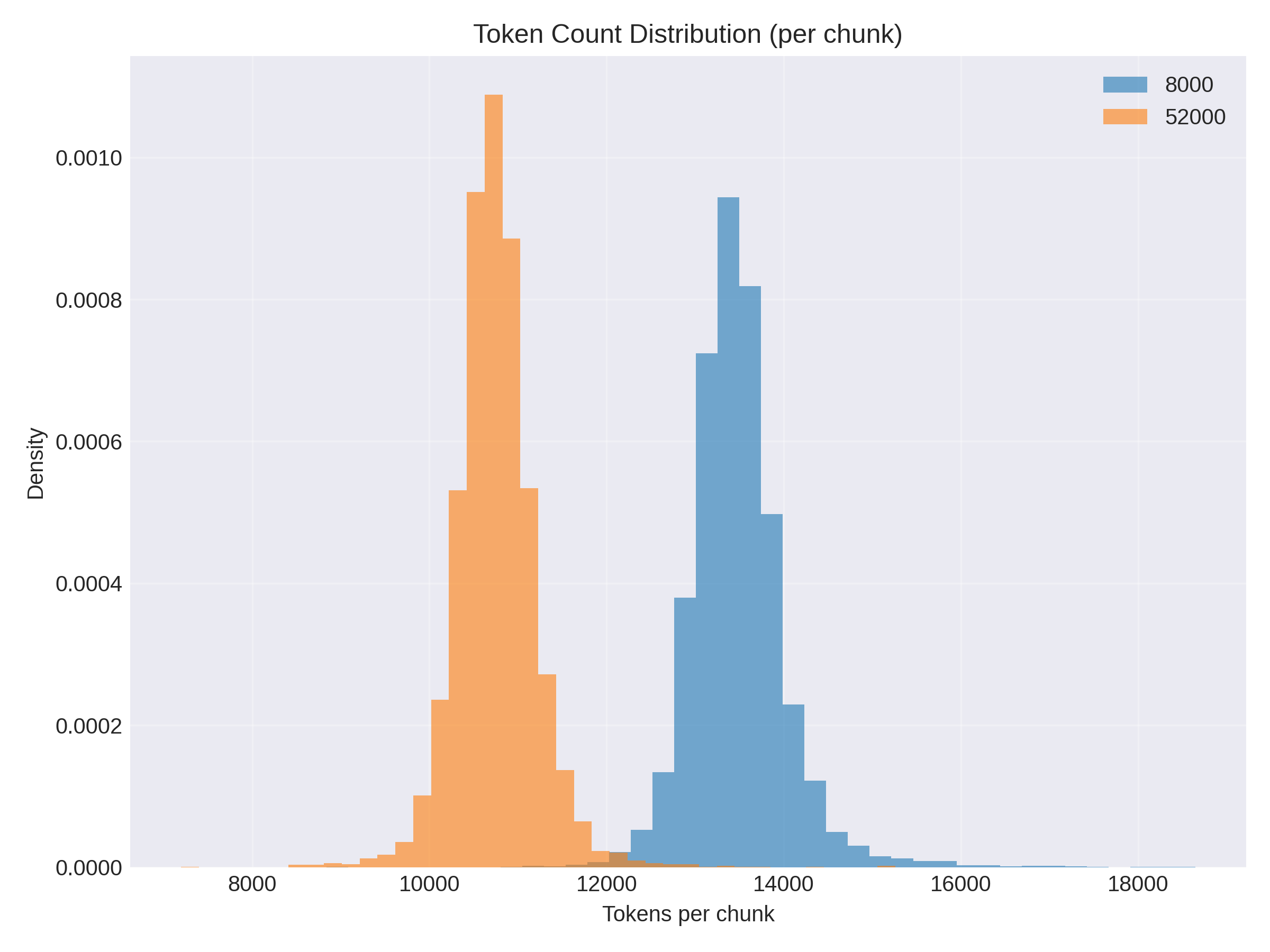
Based on this token-count distribution per chunk, you can see a clear difference: a 52k vocabulary yields better compression (average tokens per chunk is ~10.7k). With the same chunk size, using an 8k vocabulary increases the average to ~13.5k tokens.
However, that increase in tokens (around ~20%) is negligible compared to the parameter savings we can get in the Transformer, especially because, with smaller vocabularies, the embedding space can also be smaller (since we need fewer features to differentiate token meanings). This is not ideal for powerful models (bigger vocabularies and embeddings generally improve performance), but here we’re talking about small language models.
Note: There are modern ways to determine “the right” vocabulary size for a tokenizer based on the nature of the training data and this is mentioned in my LinkedIn post about Zipf’s Law.
How LLMs process tokens
Vector embeddings
After tokenizing the text, transforming human text into a sequence of predefined numbers (token_id), these tokens still need to be mapped into high-dimensional vectors called embeddings.
Let $V$ be the vocabulary size, $d$ the embedding dimension, and $C$ the context length. We learn an embedding matrix $E \in \mathbb{R}^{V \times d}$. For token IDs $x \in \mathbb{N}^C$, the lookup produces $y \in \mathbb{R}^{C \times d}$ by selecting rows of $E$.
We also learn positional embedding $P \in \mathbb{R}^{C \times d}$ to encode order. The model sums token and positional embedding: $H_0 = y + P$, and feeds $H_0$ to the attention layers.
For intuition on why this matters: the embedding space is where meaning becomes geometry. Similar words get nearby vectors (under distance functions like Euclidean distance or cosine similarity), making it easier for attention to share information across related tokens.
Positional terms ensure the model distinguishes “dog bites man” from “man bites dog.” Without these learned vectors, the model would only see arbitrary integer IDs and would lose both semantic similarity and word order, limiting its ability to reason about language.
Attention mechanism
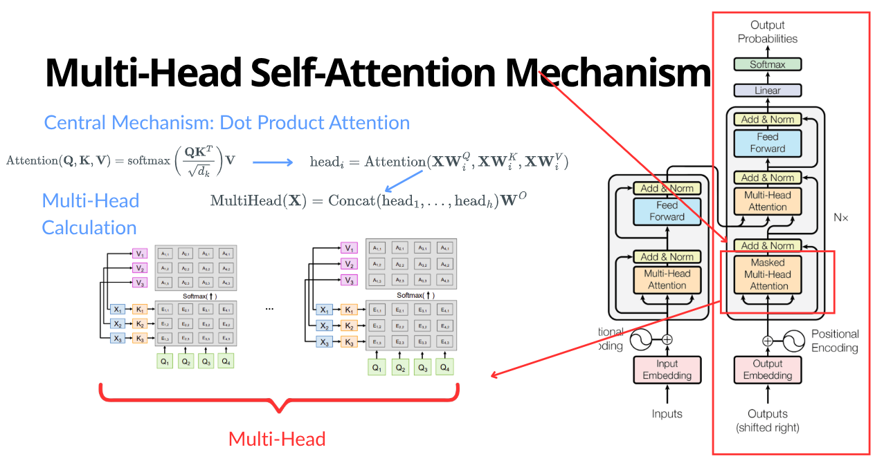
Single-head self-attention with causal masking (Vaswani et al., 2017) starts from token representations in a matrix $H_0 \in \mathbb{R}^{C \times d}$, where $C$ is the sequence length (in our case, the context length) and $d$ is the embedding dimension.
We form queries, keys, and values via $Q = H_0 W_Q,\quad K = H_0 W_K,\quad V = H_0 W_V,$ with trainable projections $W_Q, W_K, W_V \in \mathbb{R}^{d \times d}.$
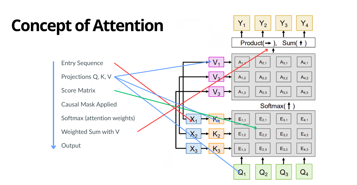
We first compute a dot product between $Q$ and $K^\top$. Intuitively, $QK^\top$ scores pairwise relevance (“how much should this token look at that token?”). The result is scaled by $\frac{1}{\sqrt{d_k}}$ (Vaswani et al., 2017), where $d_k = \frac{d}{h}$ and $d$ is the embedding dimension and $h$ is the number of attention heads). Attention heads are simply parallel attention blocks.
Why scaling is important?
But why do we scale the dot-product result? Without scaling, these dot products can explode in high dimensions. Imagine two high-dimensional random vectors: their dot product has mean 0, but variance grows linearly with dimension $d_k$. For large $d_k$, scores become overly sensitive and can range into large magnitudes $[-50, 50]$, which saturates the softmax, limits learning, and ruins gradients.
These claims can be proven mathematically and statistically. Suppose $q_i, k_i \sim \mathcal{N}(0, 1)$. Then the dot product is $s = \mathbf{q}^\top \mathbf{k} = \sum_{i=1}^{d_k} q_i k_i$. The mean remains 0, but the variance is: $$ \mathrm{Var}(s) = \mathrm{Var}\left( \sum_{i=1}^{d_k} q_i k_i \right) = \sum_{i=1}^{d_k} \mathrm{Var}(q_i k_i). $$ For each term, $\mathrm{Var}(q_i k_i) = \mathbb{E}[q_i^2]\mathbb{E}[k_i^2] = 1 \cdot 1 = 1$, and thus $\mathrm{Var}(s) = d_k$.
And here is a plot that empirically illustrates the phenomenon:
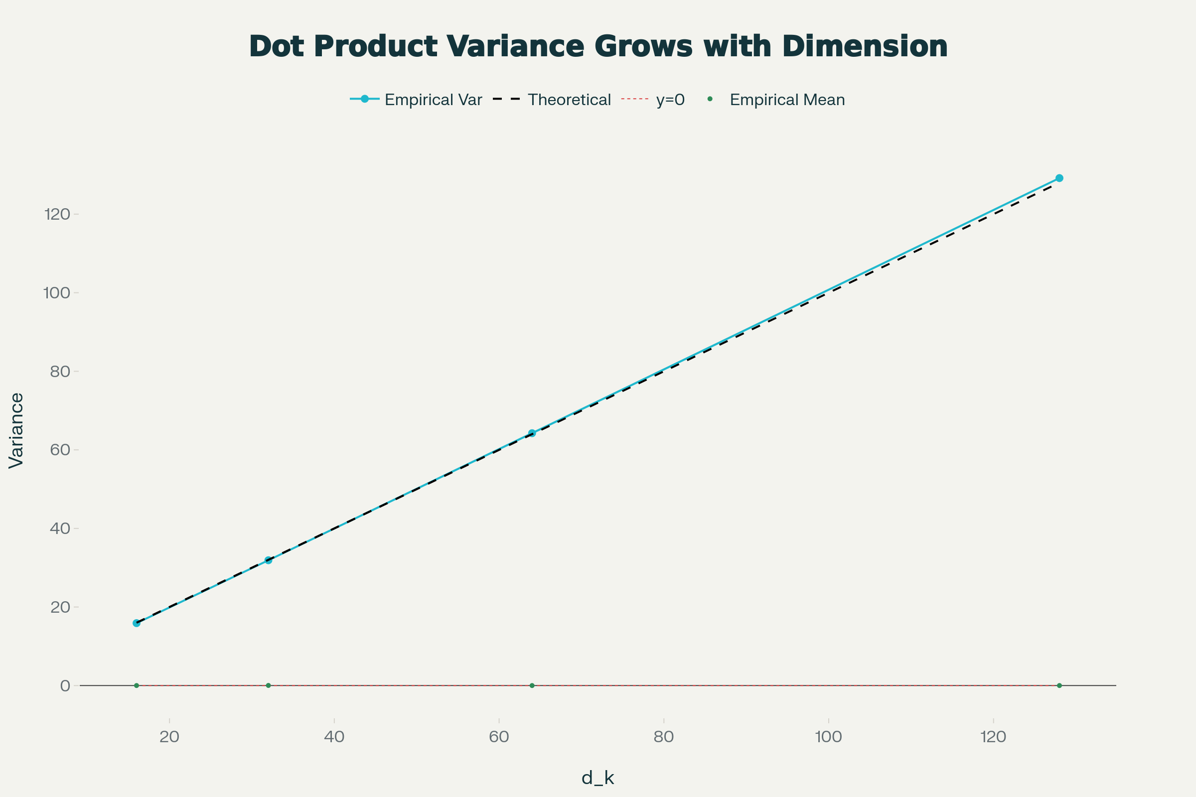
Since the variance grows linearly with $d_k$, scaling by $\frac{1}{\sqrt{d_k}}$ yields $\mathrm{Var}(A) \approx 1$, preventing softmax saturation.
Causal attention
Autoregressive LLMs like GPT generate text sequentially, token-by-token from left to right (Radford et al., 2019). They predict the next token based only on what came before, without “cheating” by peeking ahead. This mimics real language production (e.g., typing a sentence without knowing future words) and prevents information leakage during training and inference.
The causal mask $M \in \mathbb{R}^{C \times C}$ enforces that $M_{i,j} = 0$ if $j \le i$ (attend to self and past), and $-\infty$ otherwise (block the future). When added to the attention logits, it forces future probabilities to zero after the softmax: $$A = \frac{Q K^\top}{\sqrt{d_k}} + M$$ Attention weights arise from a row-wise softmax getting $W = \operatorname{softmax}(A) \in \mathbb{R}^{C \times C}.$ Each row is a probability distribution over earlier positions. Each position then aggregates values: $$C = W V \in \mathbb{R}^{C \times d},$$ producing a weighted mixture of value vectors. In multi-head attention this happens in parallel across heads (each with its own $W_Q, W_K, W_V$), the head outputs are concatenated, and an output projection may follow: $$\text{Out} = C W_O \in \mathbb{R}^{C \times d},$$ where $W_O \in \mathbb{R}^{d \times d}$ and $C$ denotes the concatenated multi-head contexts.
And here is my full implementation of the multi-head causal attention block using PyTorch:
#src/models/layers.py
class MultiHeadAttention(nn.Module):
  def __init__(self, d_in, d_out, context_length, dropout, num_heads, qkv_bias=False):
    super().__init__()
    assert d_out % num_heads == 0
    self.d_out = d_out
    self.num_heads = num_heads
    self.head_dim = d_out // num_heads
    self.W_query = nn.Linear(d_in, d_out, bias=qkv_bias)
    self.W_key = nn.Linear(d_in, d_out, bias=qkv_bias)
    self.W_value = nn.Linear(d_in, d_out, bias=qkv_bias)
    self.out_proj = nn.Linear(d_out, d_out)
    self.dropout = nn.Dropout(dropout)
    self.register_buffer("mask", torch.triu(torch.ones(context_length, context_length), diagonal=1))

  def forward(self, x):
    b, t, _ = x.shape
    k = self.W_key(x).view(b, t, self.num_heads, self.head_dim).transpose(1, 2)
    q = self.W_query(x).view(b, t, self.num_heads, self.head_dim).transpose(1, 2)
    v = self.W_value(x).view(b, t, self.num_heads, self.head_dim).transpose(1, 2)
    att = (q @ k.transpose(2, 3)) / (k.shape[-1] ** 0.5)
    m = self.mask.bool()[:t, :t]
    att = att.masked_fill(m, float("-inf"))
    w = torch.softmax(att, dim=-1)
    ctx = w @ v
    ctx = ctx.transpose(1, 2).contiguous().view(b, t, self.d_out)
    return self.out_proj(ctx)
The importance of normalization
Stacking attention and feed-forward layers often leads to training failures, similar in context to the scaling issue mentioned earlier. As the signal propagates through many layers, activation variance can explode or vanish, which leads to unstable gradients (too small to learn, or too large and divergent).
To fix this, GPT-2 utilizes Layer Normalization (LayerNorm) (Ba et al., 2016; Radford et al., 2019). LayerNorm normalizes across the feature (embedding) dimension for each sample.
Mathematically, for an input vector $x \in \mathbb{R}^d$, we first calculate the mean $\mu$ and variance $\sigma^2$ across the embedding dimension: $$ \mu = \frac{1}{d} \sum_{i=1}^d x_i $$ $$ \sigma^2 = \frac{1}{d} \sum_{i=1}^d (x_i - \mu)^2 $$ We then normalize the vector to have zero mean and unit variance (which means the variance = 1).However, it’s important to note that forcing strict normalization might limit the network’s expressiveness (as we are doing a form of compression to the internal embedding vectors).
To counter this effect, LayerNorm introduces two learnable parameters per layer $\gamma$ (scale) and $\beta$ (shift), allowing the model to “undo” the normalization if beneficial: $$ \hat{x} = \frac{x - \mu}{\sqrt{\sigma^2 + \epsilon}} $$ $$ y = \gamma \odot \hat{x} + \beta $$ Here, $\epsilon$ is a small constant (e.g., $1e^{-5}$) for numerical stability.
I implemented this layer from scratch (without relying on PyTorch’s built-in nn.LayerNorm):
#src/models/layers.py
class LayerNorm(nn.Module):
  def __init__(self, emb_dim: int):
    super().__init__()
    self.eps = 1e-5
    self.scale = nn.Parameter(torch.ones(emb_dim))
    self.shift = nn.Parameter(torch.zeros(emb_dim))
  def forward(self, x):
    mean = x.mean(dim=-1, keepdim=True)
    var = x.var(dim=-1, keepdim=True, unbiased=True)
    x = (x - mean) / torch.sqrt(var + self.eps)
    return self.scale * x + self.shift
For my implementation, I followed the GPT-2 pre-norm formulation (Radford et al., 2019), which applies LayerNorm before the sub-layers: $$ x_{l+1} = x_l + F(\text{LayerNorm}(x_l)) $$
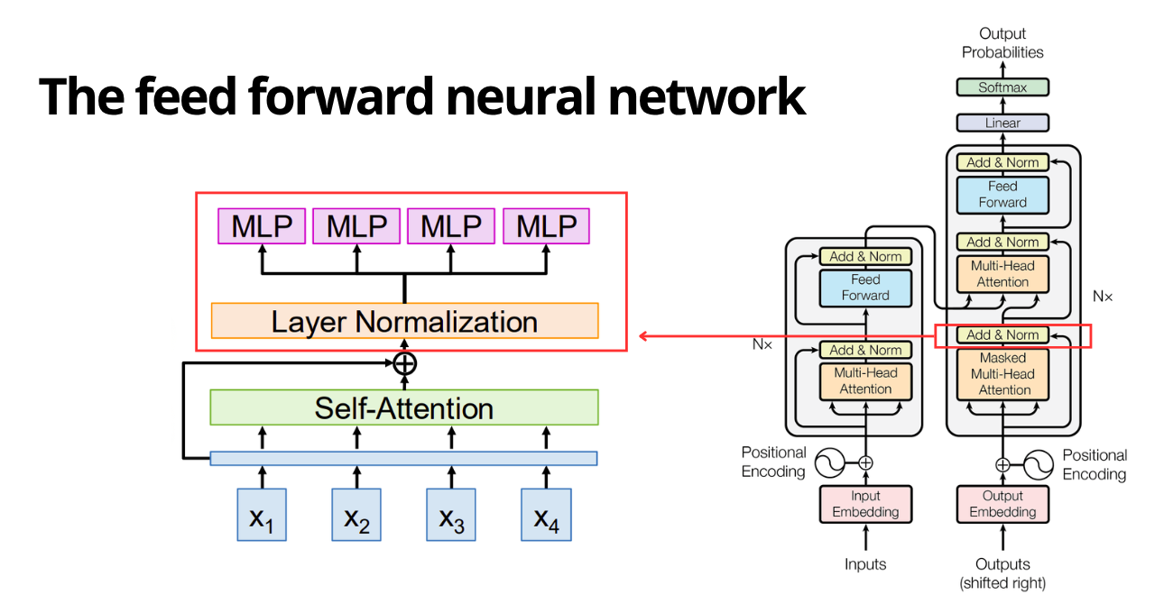
The feed forward neural network
Self-attention’s role is to aggregate information across token positions through weighted combinations, while the feed-forward network (FFN) applies non-linear transformations independently to each token’s representation (embedding).
I used the standard GPT architecture, which is a simple Multi-Layer Perceptron (MLP) applied position-wise. This means the exact same weights are applied to every token in the sequence, effectively in parallel.
Dimensional Expansion:
An important design choice in Transformers is the expansion factor (Vaswani et al., 2017). The input projects from embedding dimension $d$ to a hidden dimension $4d$, and then back down to $d$. $$ \text{FFN}(x) = \text{GELU}(x W_1 + b_1) W_2 + b_2 $$ Where $W_1 \in \mathbb{R}^{d \times 4d}$ and $W_2 \in \mathbb{R}^{4d \times d}$.
The interesting part about this expansion is that by projecting the data into a higher-dimensional space, we give the model more capacity to decouple overlapping features and learn complex, non-linear functions. However, this layer also holds the majority of the model’s parameters (roughly ~2/3 of the total), so it represents much of the model’s internal “knowledge” capacity.
But why are we using GELU?
For the non-linearity component, the standard for GPT-2, BERT, and many modern LLMs is GELU instead of ReLU (Hendrycks & Gimpel, 2016). This choice is supported by the following intuition:
GELU is used because it behaves like a “soft” version of ReLU that keeps gradients non-zero (very small values near zero or even negative values still carry information, unlike hard zeros).

The problem ReLU has with hard zeros is that when negative values appear, ReLU maps them to 0, meaning no gradient for those activations. This can cause parts of the network to stop learning, a failure mode called “dying ReLU.”
GELU, on the other hand, is smoother. It weights the input $x$ by how likely it is to be on the positive side under a normal distribution. If the value is small or negative, it’s downweighted rather than completely removed.
During training, since gradients come from derivatives, GELU’s smoothness provides a continuous derivative, which tends to make optimization more stable.
The original mathematical expression is:
$$ \text{GELU}(x) = x \cdot \Phi(x) $$
Where $\Phi(x)$ is the cumulative distribution function of the standard normal distribution. Intuitively, it attenuates inputs depending on their magnitude. Since computing the exact ERF is expensive, we often use the approximation:
$$ \text{GELU}(x) \approx 0.5x \left( 1 + \tanh \left[ \sqrt{\frac{2}{\pi}} (x + 0.044715 x^3) \right] \right) $$
I implemented the previous concepts using PyTorch’s nn.Sequential since it’s a sequence of layers rather than a single layer.
#src/models/layers.py
class FeedForward(nn.Module):
  def __init__(self, emb_dim: int):
    super().__init__()
    self.layers = nn.Sequential(
      nn.Linear(emb_dim, 4 * emb_dim),
      GELU(),
      nn.Linear(4 * emb_dim, emb_dim),
    )
  def forward(self, x): return self.layers(x)
LLM pre-training
Pre-training is the fundamental phase where the LLM learns the structure of language and acquires general knowledge. While we often think of “training” as teaching a model a specific task (like sentiment analysis), pre-training is different. Its goal isn’t to solve a specific problem, but to act as a compression algorithm for the training corpus. By learning to predict the next word, the model effectively internalizes the grammar, facts, and reasoning patterns found in the data.
How self-supervised learning works in LLMs
You might hear the term “unsupervised learning” thrown around for LLMs, but more accurately it is self-supervised learning. The training signal is created directly from raw data, eliminating the need for expensive human annotation.
The core task is Next Token Prediction. We feed the model a sequence of text and ask it to predict the very next token. If the model guesses correctly, we reward it; if not, we adjust the weights.
The “Sliding Window” Strategy
In my implementation, I treat the raw text (from the FineWeb dataset) (Penedo et al., 2024) as one massive stream of tokens. To create training examples, I use a sliding window approach.

For a context length $L$, we take a chunk of text. The input is the sequence from index $0$ to $L-1$, and the target (the “label”) is the sequence from index $1$ to $L$.
This effectively shifts the target by one position to the right. Here is the logic I implemented in GPTDatasetV1:
# src/data/datasets.py
# Create sliding windows with stride
for sequence_start_index in range(0, len(tokenized_text) - max_length, stride):
    # Input: tokens [t_0, ..., t_{L-1}]
    input_sequence = tokenized_text[sequence_start_index : sequence_start_index + max_length]

    # Target: tokens [t_1, ..., t_L] (Shifted by one)
    target_sequence = tokenized_text[sequence_start_index + 1 : sequence_start_index + max_length + 1]

    self.input_sequences.append(torch.tensor(input_sequence))
    self.target_sequences.append(torch.tensor(target_sequence))
A single window of length $L$ provides $L$ distinct training examples (one for every position in the sequence) simultaneously.
But we still need to define how we reward and punish the model.
The objective function (cross-entropy)
Mathematically, we want to maximize the likelihood of the correct token $x_t$ given the previous tokens $x_{<t}$. This is equivalent to minimizing the negative log-likelihood (cross-entropy loss):
$$ \mathcal{L} = - \sum_{t=1}^{L} \log P(x_t \mid x_{<t}; \theta) $$
In PyTorch, this is straightforward, but there is a dimensional issue. The model’s output logits have shape (batch_size, context_length, vocab_size). For example, with a batch of 4 sequences, a context length of 128 tokens, and a vocabulary of 50,257 tokens, you get (4, 128, 50257).
However, torch.nn.functional.cross_entropy expects an input 2D tensor of shape (N, C), where $N$ is the number of samples and $C$ is the number of classes, and a target 1D tensor of shape (N,) containing class indices.
The key idea is that in language modeling, every token prediction is an independent classification task. When we have 4 sequences of 128 tokens each, we are making $4 \times 128 = 512$ separate predictions, each choosing one token from a 50,257-token vocabulary.
By flattening (4, 128, 50257) to (512, 50257), we are treating all 512 token positions across all sequences as 512 independent classification problems, each with 50,257 classes.
And here is an implementation example using PyTorch:
# src/training/evaluate.py
def calc_loss_batch(input_batch, target_batch, model, device):
    logits = model(input_batch)
    # Flatten (Batch, Time, Vocab) -> (Batch * Time, Vocab)
    return torch.nn.functional.cross_entropy(
        logits.flatten(0, 1),
        target_batch.flatten()
    )
By minimizing this loss over millions of iterations, the model moves from outputting random noise to generating coherent, fluent English.
Estimating data volume (Chinchilla)
One of the most common mistakes when training LLMs is guessing the dataset size. Train on too little data, and your model is “undertrained” (it has the capacity to learn more but hasn’t seen enough examples). Train on too much, and you are wasting compute resources for diminishing returns.
But how do we find the sweet spot? The Chinchilla scaling laws (Hoffmann et al., 2022) addressed this question with an experimental heuristic.
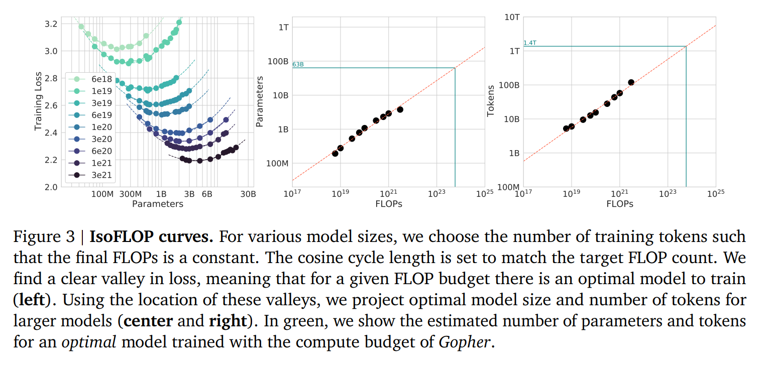
The core finding of the Chinchilla paper is that for a given compute budget, the model size ($N$) and the number of training tokens ($D$) should scale equally. The golden rule of thumb derived from their extensive experiments is a 20:1 ratio: $$ D \approx 20 \times N $$ For every model parameter, you need roughly 20 tokens of text to train it effectively.
However, in my current implementation, the model size is approximately 35 million parameters. Based on the paper, the optimal (recommended) number of training tokens is around 700 million.
But unfortunately, my dataset contains around 66 million tokens, so my current ratio is around 1.9 tokens per parameter. This suggests my model is severely undertrained according to Chinchilla optimality.
To reach its full potential, I would need a dataset 10x larger. However, training on 700M tokens on a single RTX 3050 would take days rather than hours. This is a deliberate trade-off: I accepted “undertraining” to complete the project faster, since it’s only a proof of concept.
Quantity isn’t quality
Even if you hit the 20:1 ratio, the composition of the data matters just as much. A model trained purely on Wikipedia will be great at facts but terrible at conversation. A model trained only on Reddit might be conversational but prone to toxicity and hallucinations.
For a small language model (SLM), dataset engineering is critical: you want diverse, high-quality data with a mixture of narrative, conversational, and factual text.
FineWeb contains many of the characteristics of a good dataset for small language model training. However, because the volume of data I used isn’t large, that likely explains why my model hallucinates so much.
Preparing the dataset
Before training, the raw text must be transformed into a format the model can consume. In PyTorch, this is handled by two core components: the Dataset, which defines how to read a single example, and the DataLoader, which batches these examples together for the GPU.
The GPTDatasetV1 Implementation
For pre-training, I built a custom Dataset class that essentially converts a massive string of text into a sliding window of tokens. The key challenge here is memory efficiency. Instead of pre-slicing the text into millions of small strings (which would blow up RAM), I tokenize the entire dataset once and store it as a single tensor.
During training, the __getitem__ method simply slices this master tensor on the fly:
#src/data/datasets.py
class GPTDatasetV1(Dataset):
    def __init__(self, text, tokenizer, max_length, stride):
        self.tokenizer = tokenizer
        self.input_ids = []
        self.target_ids = []

        # Tokenize the entire text once
        token_ids = tokenizer.encode(text, allowed_special={"<|endoftext|>"})

        # Slide a window across the text with a stride
        for i in range(0, len(token_ids) - max_length, stride):
            input_chunk = token_ids[i : i + max_length]
            target_chunk = token_ids[i + 1 : i + max_length + 1]

            self.input_ids.append(torch.tensor(input_chunk))
            self.target_ids.append(torch.tensor(target_chunk))

    def __len__(self):
        return len(self.input_ids)

    def __getitem__(self, idx):
        return self.input_ids[idx], self.target_ids[idx]
The stride parameter is important here, as it determines how much overlap exists between training examples. A smaller stride generally means more data augmentation (seeing the same sentence in different positions), but it also costs more training time.
Cleaning Techniques for Small Models
When training a model with only ~35M parameters, data quality is far more important than quantity. Large models can learn to ignore noise because it averages out across massive datasets; small models tend to be affected by noise because they don’t have as much capacity (or data) to wash it out.
Although my implementation used relatively raw text from FineWeb, I still did some preprocessing to improve data quality:
- First, I applied basic normalization (e.g., NFC normalization) to convert text into a consistent format. This prevents the tokenizer from treating the same word as different tokens due to special characters.
- I also inserted a special token (
<|endoftext|>) between documents/samples. Without this, the model might learn to merge the end of a Wikipedia article about quantum physics directly into the start of a recipe for apple pie, confusing its internal state. This token teaches the LLM when to stop and reset between topics.
In my case, I relied on the tiktoken tokenizer (the original GPT-2 BPE) (Radford et al., 2019; Sennrich et al., 2016).
Training process
Training an LLM is a balancing act between mathematical optimality, stability, and computational constraints. With a single low-end GPU such as an NVIDIA RTX 3050 with 4GB of VRAM, training becomes harder, which calls for a few optimization techniques.
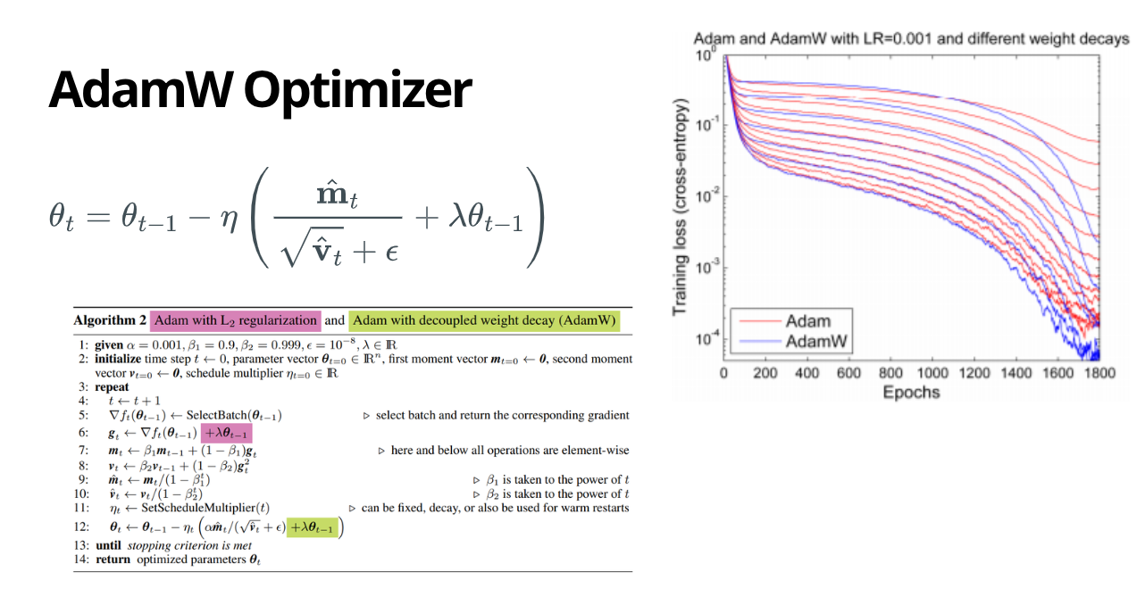
Using the AdamW optimizer (Kingma & Ba, 2014; Loshchilov & Hutter, 2017)
Standard stochastic gradient descent (SGD) is usually slow and much more sensitive to learning-rate tuning; it’s also notorious for becoming unstable early in training. It requires a carefully tuned learning rate that is often dynamic, which is why it’s not the default choice for training LLMs.
However, AdamW adapts the learning rate for every single parameter individually. If a parameter receives large gradients (is changing a lot), AdamW slows it down; if it receives small updates (is rarely used), AdamW speeds it up.
I used PyTorch’s native implementation, enabling the fused=True flag to run the entire optimization step as a single CUDA kernel, speeding up gradient calculations:
# src/training/trainer.py
optimizer = torch.optim.AdamW(
    model.parameters(),
    lr=5e-4,              # Peak learning rate
    betas=(0.9, 0.95),    # Control momentum
    eps=1e-8,             # Stability term
    weight_decay=0.1,     # Regularization to prevent overfitting
    fused=True            # CUDA optimization
)
LLMs need batch processing (and Gradient Accumulation)
For the training to be stable, the “batch size” needs to be large. A large batch provides a statistically accurate estimate of the true gradient, filtering out the noise of individual random sentences.
However, a large batch size requires massive VRAM. On my 4GB GPU, I could only fit a micro-batch size of roughly 4 examples. Updating weights every 4 examples would make the training unstable.
The solution is gradient accumulation. Instead of updating the weights after every forward pass, we accumulate gradients over several small steps. We run the forward and backward passes multiple times, add up the gradients, and only then take an optimizer step.
In the training loop, this looks like simulating a large batch sequentially:
# Virtual Batch Size = batch_size * grad_accum_steps
for i, (inputs, targets) in enumerate(dataloader):
    # 1. Calculate loss for this micro-batch
    logits = model(inputs)
    loss = F.cross_entropy(logits, targets)

    # 2. Scale loss to average it over the accumulation steps
    loss = loss / grad_accum_steps
    loss.backward()  # Accumulate gradients

    # 3. Step only after N micro-batches
    if (i + 1) % grad_accum_steps == 0:
        optimizer.step()
        optimizer.zero_grad()
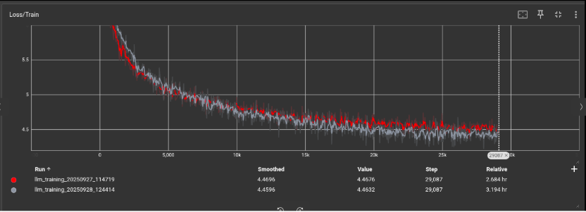
This allowed me to simulate a batch size of 32 or 64, which helped me approximate the stability you’d normally get with much larger hardware. The tradeoff is longer training time per optimizer step.
And here is an image of the evolution of loss:
The problem with fixed learning rate
Training with a constant learning rate usually leads to one of two outcomes: a high learning rate makes the model learn quickly at first but diverge later; a low learning rate keeps training stable but takes too long to learn anything useful.
But didn’t we say AdamW controls step sizes (learning rates)? Why do we still need additional control?
AdamW and the learning-rate schedule solve different parts of the same optimization problem. AdamW adapts update sizes per parameter, while the schedule controls the global scale of all those updates over time.
In AdamW, the parameter update is still multiplied by the base learning rate, the “adaptive” part mainly rescales each parameter’s step using running gradient statistics.
So the schedule is effectively a time-varying adjustments that scales all AdamW updates together.
Learning-rate scheduling (warmup and cosine annealing)
To get a good learning-rate schedule, I used two complementary techniques:
Linear Warmup: Early in training, AdamW’s moment estimates (moving averages of gradients) are not well-formed yet, and gradients can be unusually large or noisy.
Warmup starts with tiny steps so those statistics stabilize before the optimizer is allowed to take full-size updates, which reduces sudden loss spikes.
Cosine Decay: As training progresses, the goal changes from “move quickly toward a good region” to “fine-tune inside that region.” Cosine decay gradually lowers the base learning rate (Loshchilov & Hutter, 2016), shrinking AdamW’s effective step sizes so updates become more precise and training becomes less jittery near convergence.
I combined these using PyTorch’s SequentialLR:
# 1. Warmup from 0 to max_lr
warmup = LinearLR(optimizer, start_factor=1e-8, total_iters=warmup_steps)
# 2. Decay from max_lr to min_lr
decay = CosineAnnealingLR(optimizer, T_max=total_steps - warmup_steps)
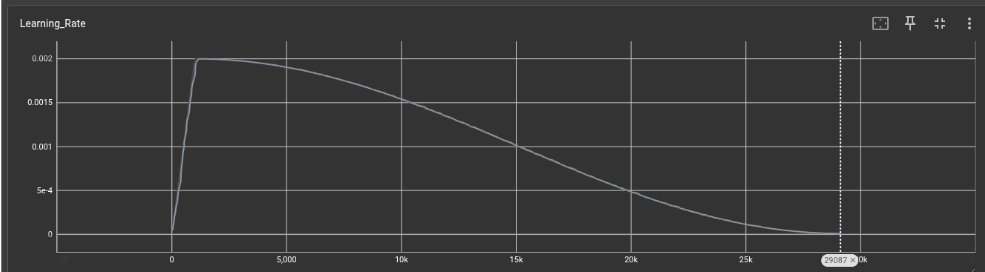
scheduler = SequentialLR(optimizer, schedulers=[warmup, decay], milestones=[warmup_steps])
You can see the learning-rate schedule below (plotted with TensorBoard):
Instruction fine-tuning
After hours of pre-training, I had a model that could speak fluent English. But if I asked it, “Who is the president of the US?”, it confidently produced the following:
Once upon a time. He was a member. He was a municipality in the "Theborn. He was a municipality in the United States. He was a municipality in the United in the United in the United of the United...
Why fine-tuning is important
You can see the model is generating good English, but the content is garbage. It identified that we’re talking about a person by saying He was, and it associated “US” with municipality and United States. There are also weird repetitions like in the United in the United of the United (which we’ll address later with sampling methods). But the core question still isn’t answered.
This happens because a pre-trained LLM is an unfiltered probabilistic engine. It doesn’t know what a “question” or an “instruction” is; it only knows how to statistically predict the next word based on patterns in its training data (web pages, books, articles).
At this stage, the model is just a text completion machine. If you write an instruction, the model thinks you’re starting a document and will try to finish it in the same style. To turn this “document completer” into a helpful assistant, we need instruction fine-tuning.
Alpaca instruction fine-tuning
To bridge the gap between “text completion” and “instruction following,” I adopted the methodology pioneered by the Stanford Alpaca project (Taori et al., 2023). Their work demonstrated that a small, weak model (like mine) can behave like a much larger one (like GPT-3) if it is fine-tuned on high-quality instruction-response pairs.
This process, often called Supervised Fine-Tuning (SFT), forces the model to align its probabilistic distribution with specific task-oriented behaviors.
The data format
The training data is structured in a JSON format containing three fields:
- Instruction: The task description (e.g., “Give me a recipe for pancakes”).
- Input: Optional context (e.g., specific ingredients to use).
- Output: The desired answer.
However, the model cannot read JSON directly. We must flatten this structured data into a single string that mimics a conversation. In this project, I used the standard Alpaca prompt template:
### Instruction:
{instruction}

### Input:
{input}

### Response:
{output}<|endoftext|>
Masked loss
The most critical technical implementation in SFT is Loss Masking.
In standard pre-training, the model learns from every token. However, during fine-tuning, we don’t want the model to “learn” the instruction. The instruction is given by the user; the model’s job is only to generate the response.
If we calculated loss on the entire sequence, the model would waste gradient updates learning to memorize the static string ### Instruction:. To prevent this, we need to effectively remove the loss for the prompt.
We create a binary mask vector $M$ of the same length as the token sequence:
- $M_i = 0$ for all tokens in the Prompt (Instruction + Input).
- $M_i = 1$ for all tokens in the Response (Output).
Mathematically, the standard cross-entropy loss is modified to: $$ \mathcal{L} = \frac{\sum_{t} \mathcal{L}_{CE}(\hat{y}t, y_t) \cdot M_t}{\sum{t} M_t} $$ This masked cross-entropy loss is implemented in PyTorch as follows:
# Create a mask: 0 for prompt, 1 for response
mask = torch.tensor(
    [0] * len(prompt_tokens) + [1] * len(response_tokens),
    device=loss.device,
    dtype=loss.dtype,
)

# ... inside training loop ...

# Calculate standard loss (element-wise)
loss = F.cross_entropy(logits, targets, reduction='none')

# Multiply by the mask to zero-out prompt loss
masked_loss = loss * mask

# Normalize by the number of valid tokens (prevent division by zero)
final_loss = masked_loss.sum() / mask.sum().clamp_min(1)
By filtering out the prompt, 100% of the model’s learning capacity is focused on generating better answers rather than memorizing the instruction boilerplate.
After training the model on the Alpaca dataset (around 50k examples) (Taori et al., 2023), here are a few examples from the data:
[
    {
        "instruction": "Give three tips for staying healthy.",
        "input": "",
        "output": "1.Eat a balanced diet and make sure to include plenty of fruits and vegetables. \n2. Exercise regularly to keep your body active and strong. \n3. Get enough sleep and maintain a consistent sleep schedule."
    },
    {
        "instruction": "What are the three primary colors?",
        "input": "",
        "output": "The three primary colors are red, blue, and yellow."
    },
    ...
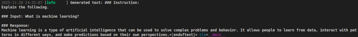
We’re finally able to get some serious answers from an undertrained LLM. When I asked the model What is machine learning?, look at the answer:
Machine learning is a type of artificial intellgience that can be used to solve complex problems and behavior. It allows people to learn from data, interact with patterns in different ways, and make predictions based on their own perspectives.<|endoftext|>
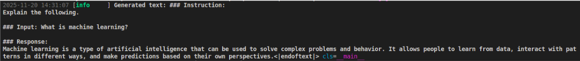
The answer is not perfect, but I’m proud that the model is finally able to generate such a response.
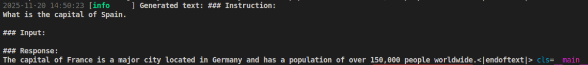
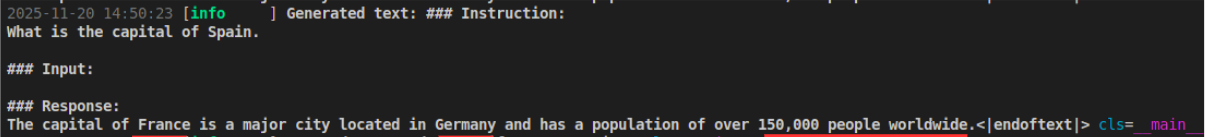
But the model is still far from perfect—it gave the following answer to What is the capital of Spain?:
The capital of France is a major city located in Germany and has a population of over 150,000 people worldwide.<|endoftext|>
The importance of sampling
Even with a perfectly trained model, the way you select the next word can ruin everything. When I first ran my model using simple “Greedy Decoding” (always picking the most likely next word), I asked it: “Who is the president of the US?” And as previously mentioned, I got this output:
Once upon a time. He was a member. He was a municipality in the "Theborn. He was a municipality in the United States. He was a municipality in the United in the United in the United of the United...
LLMs are weird without sampling
This repetition loop is a classic failure mode of deterministic decoding. When the model is uncertain, it often assigns the highest probability to safe, common words like “the” or “United.” Once it outputs one, the probability of seeing it again slightly increases, creating a positive feedback loop that traps the model in a cycle of “United in the United in the United.”
To fix this, we must stop always picking the “best” word and start sampling from “likely” words. This introduces sampling, and the first sampling technique is temperature.
Temperature
The most important parameter to tune is temperature ($T$). Before we convert the model’s output scores (logits) into probabilities (softmax), we divide them by $T$: $$ P_i = \frac{\exp(z_i / T)}{\sum_j \exp(z_j / T)} $$ The choice of the $T$ value creates drastically different behaviors:
- Low Temperature ($T < 1.0$): Exaggerates differences. The “best” token gets 99% probability. The model becomes conservative, factual, and repetitive.
- High Temperature ($T > 1.0$): Flattens the curve. Rare words gets more attention. The model becomes creative, diverse, but prone to hallucinations.
The implementation is straightforward in Python:
# src/training/generate.py
if temperature > 0:
    logits = logits / temperature

probs = F.softmax(logits, dim=-1)
next_id = torch.multinomial(probs, num_samples=1)
Top-k and Top-p
Even with temperature, the model might occasionally pick a statistically valid but contextually nonsensical word (like “banana” appearing in a sentence about politics). To prevent this, we truncate the tail of the distribution.
- Top-k: We only sample from the top $k$ most likely tokens (e.g., top 50). This severely cuts off the long tail of nonsense.
- Top-p (Nucleus): Instead of a fixed number, we dynamically select the smallest set of tokens whose cumulative probability exceeds $p$ (e.g., 0.95).
If the model is certain (e.g., “The cat sat on the…”), the top 0.95 might just be one word (“mat”). If it is uncertain, the top 0.95 might include 100 verbs. This adapts the “creativity” to the model’s own confidence level.
And here is my implementation of both approaches:
# src/training/generate.py
def _top_k_top_p_filtering(logits, top_k=0, top_p=0.0):
    if top_k > 0:
        # Keep only top k tokens, set others to -inf
        val, _ = torch.topk(logits, top_k)
        logits[logits < val[:, [-1]]] = float('-inf')

    if top_p > 0.0:
        # Sort logits and compute cumulative probs
        sorted_logits, sorted_indices = torch.sort(logits, descending=True)
        cumulative_probs = torch.cumsum(F.softmax(sorted_logits, dim=-1), dim=-1)

        # Remove tokens with cumulative probability above the threshold
        sorted_mask = cumulative_probs > top_p
        # Shift mask right to keep at least one token
        sorted_mask[..., 1:] = sorted_mask[..., :-1].clone()
        sorted_mask[..., 0] = False
        # Scatter back to original token indices
        mask = torch.zeros_like(logits, dtype=torch.bool).scatter(1, sorted_indices, sorted_mask)
        logits[mask] = float('-inf')

    return logits
Repetition penalties
Despite these mathematical tricks, small models still love to repeat themselves—like the earlier example in the United in the United in the United of the United. To fix this, I implemented a repetition penalty that lowers the logits of any token that has already appeared in the sequence using some n-gram tricks:
# src/training/generate.py
def _apply_repetition_penalty(logits, generated, penalty):
    # Get unique tokens already generated
    unique_tokens = torch.unique(generated)

    # Divide positive logits by penalty (lowering probability)
    # Multiply negative logits by penalty (making them more negative)
    logits[:, unique_tokens] /= penalty
    return logits
This simple algorithmic constraint, combined with banning specific 3-gram repetitions, was the final key that turned He was a municipality in the United in the United into coherent, fluent English.
References
Ba, J. L., Kiros, J. R., & Hinton, G. E. (2016). Layer Normalization. arXiv preprint arXiv:1607.06450.
Hendrycks, D., & Gimpel, K. (2016). Gaussian Error Linear Units (GELUs). arXiv preprint arXiv:1606.08415.
Hoffmann, J., Borgeaud, S., Mensch, A., Buchatskaya, E., Cai, T., Rutherford, E., … & Sifre, L. (2022). Training Compute-Optimal Large Language Models. arXiv preprint arXiv:2203.15556.
Holtzman, A., Buys, J., Du, L., Forbes, M., & Choi, Y. (2019). The Curious Case of Neural Text Degeneration. arXiv preprint arXiv:1904.09751.
Kingma, D. P., & Ba, J. (2014). Adam: A Method for Stochastic Optimization. arXiv preprint arXiv:1412.6980.
Loshchilov, I., & Hutter, F. (2016). SGDR: Stochastic Gradient Descent with Warm Restarts. arXiv preprint arXiv:1608.03983.
Loshchilov, I., & Hutter, F. (2017). Decoupled Weight Decay Regularization. arXiv preprint arXiv:1711.05101.
OpenAI. (2023). tiktoken: A fast BPE tokenizer for OpenAI models (software). GitHub repository: https://github.com/openai/tiktoken.
Penedo, G., Kydlíček, H., Ben Allal, L., Lozhkov, A., Mitchell, M., Raffel, C., Von Werra, L., & Wolf, T. (2024). The FineWeb Datasets: Decanting the Web for the Finest Text Data at Scale. arXiv preprint arXiv:2406.17557.
Radford, A., Wu, J., Child, R., Luan, D., Amodei, D., & Sutskever, I. (2019). Language Models are Unsupervised Multitask Learners. OpenAI. https://cdn.openai.com/better-language-models/language_models_are_unsupervised_multitask_learners.pdf
Raschka, S. (2024). Build a Large Language Model (From Scratch). Manning Publications.
Sennrich, R., Haddow, B., & Birch, A. (2016). Neural Machine Translation of Rare Words with Subword Units. In Proceedings of ACL 2016.
Stanford CS231n. (n.d.). CS231n: Deep Learning for Computer Vision — Lecture 8: Attention and Transformers (course slides). https://cs231n.stanford.edu/slides/2025/lecture_8.pdf
Taori, R., Gulrajani, I., Zhang, T., Dubois, Y., Li, X., Guestrin, C., Liang, P., & Hashimoto, T. B. (2023). Alpaca: A Strong, Replicable Instruction-Following Model. Stanford Center for Research on Foundation Models. https://crfm.stanford.edu/2023/03/13/alpaca.html
Vaswani, A., Shazeer, N., Parmar, N., Uszkoreit, J., Jones, L., Gomez, A. N., Kaiser, Ł., & Polosukhin, I. (2017). Attention Is All You Need. In Advances in Neural Information Processing Systems (NeurIPS 2017). arXiv preprint arXiv:1706.03762.